Scaling up the training data
The last installment left off with both the first- and second-order models showing a powerful thirst for more training data. After consideration, I realized that for the types of errors I want the proofreader to identify aren't unique to sci-fi books. The basics of spelling and grammar are mostly the same across all English prose.
It took a little time to figure out how to properly download Project Gutenberg texts at scale, but I finally set up three new training corpuses:
- All the English science fiction texts I could gather (2,032 books)
- All the English fiction texts I could gather (14,382 books)
- All the English texts I could gather (38,673 books)
These were used to train three different first-order models that were otherwise identical.
| version | model | description | tokenizer | alphabet | books | error cutoff |
|---|---|---|---|---|---|---|
| 19 | 04 | Sparse 1st-order Markov | 05 | 20k | 2032 | 1e-08 |
| 20 | 05 | Sparse 1st-order Markov | 05 | 20k | 14382 | 1e-08 |
| 22 | 07 | Sparse 1st-order Markov | 05 | 20k | 38673 | 1e-08 |
With these results across the four existing evals.
| version | capitalization | grammar | punctuation | spelling |
|---|---|---|---|---|
| 19 | (15) 56 | (22) 66 | (12) 42 | (19) 70 |
| 20 | (30) 20 | (54) 30 | (33) 18 | (35) 24 |
| 22 | (47) 14 | (59) 20 | (36) 10 | (31) 10 |
Performance values are shown as: (precision %) recall %
As the amount of training text increased, so did the precision. If the model noticed something surprising, it was more likely to be an actual error if the model had a larger training corpus. The more text the model had seen, the better it got at only finding errors.
On the flip side, the more training data a model had, the more likely it was to dismiss an error because it had seen it somewhere before. Legitmate errors were skipped over. Recall got lower as training corpuses got larger.
The effect of error thresholds
This is a good thing! By increasing the error threshold from near zero, it's possible to adjust the trade-off between precision and recall. As the error threshold gets higher, it raises the bar for what the model considers normal. Even if a pattern has occurred once already, it can still be tagged as an error.
This is illustrated by taking version 22, the first-order model trained on all Project Gutenburg English texts, and comparing to a collection of other models with varying error thresholds.
| version | model | description | tokenizer | alphabet | books | error cutoff |
|---|---|---|---|---|---|---|
| 22 | 07 | Sparse 1st-order Markov | 05 | 20k | 38673 | 1e-08 |
| 27 | 07 | Sparse 1st-order Markov | 05 | 20k | 38673 | 1e-07 |
| 23 | 07 | Sparse 1st-order Markov | 05 | 20k | 38673 | 1e-06 |
| 28 | 07 | Sparse 1st-order Markov | 05 | 20k | 38673 | 1e-05 |
| 24 | 07 | Sparse 1st-order Markov | 05 | 20k | 38673 | 0.0001 |
| 25 | 07 | Sparse 1st-order Markov | 05 | 20k | 38673 | 0.001 |
| 26 | 07 | Sparse 1st-order Markov | 05 | 20k | 38673 | 0.01 |
| version | capitalization | grammar | punctuation | spelling |
|---|---|---|---|---|
| 22 | (47) 14 | (59) 20 | (36) 10 | (31) 10 |
| 27 | (50) 16 | (61) 22 | (36) 10 | (31) 10 |
| 23 | (55) 22 | (67) 32 | (39) 14 | (39) 14 |
| 28 | (33) 32 | (61) 46 | (27) 28 | (30) 28 |
| 24 | (16) 70 | (20) 74 | (16) 70 | (15) 64 |
| 25 | (8) 98 | (10) 96 | (9) 98 | (8) 100 |
| 26 | (5) 98 | (6) 100 | (5) 100 | (5) 100 |
As the error threshold moves from 10^-8 to 10^-2, the performance changes dramatically. Initially at 10^-8, both precision and recall climb. Then at around 10^-6 precision tops out, while recall continues to climb. 10^-5 is a good point for balancing precision's fall with recall's climb. 10^-4 has respectable recall values across the board, with precision being around 1 in 6. After that we see the patterns of earlier. Precision falls into the single digits while recall jumps up to 100. The model starts to shotgun tag anything that is less than common.
Reporting in pictures
The tables above and the paragraph of explanation that follows require a lot of mental steps to stitch together into a story. This is why plots were invented.
Here is the same information, reformatted.
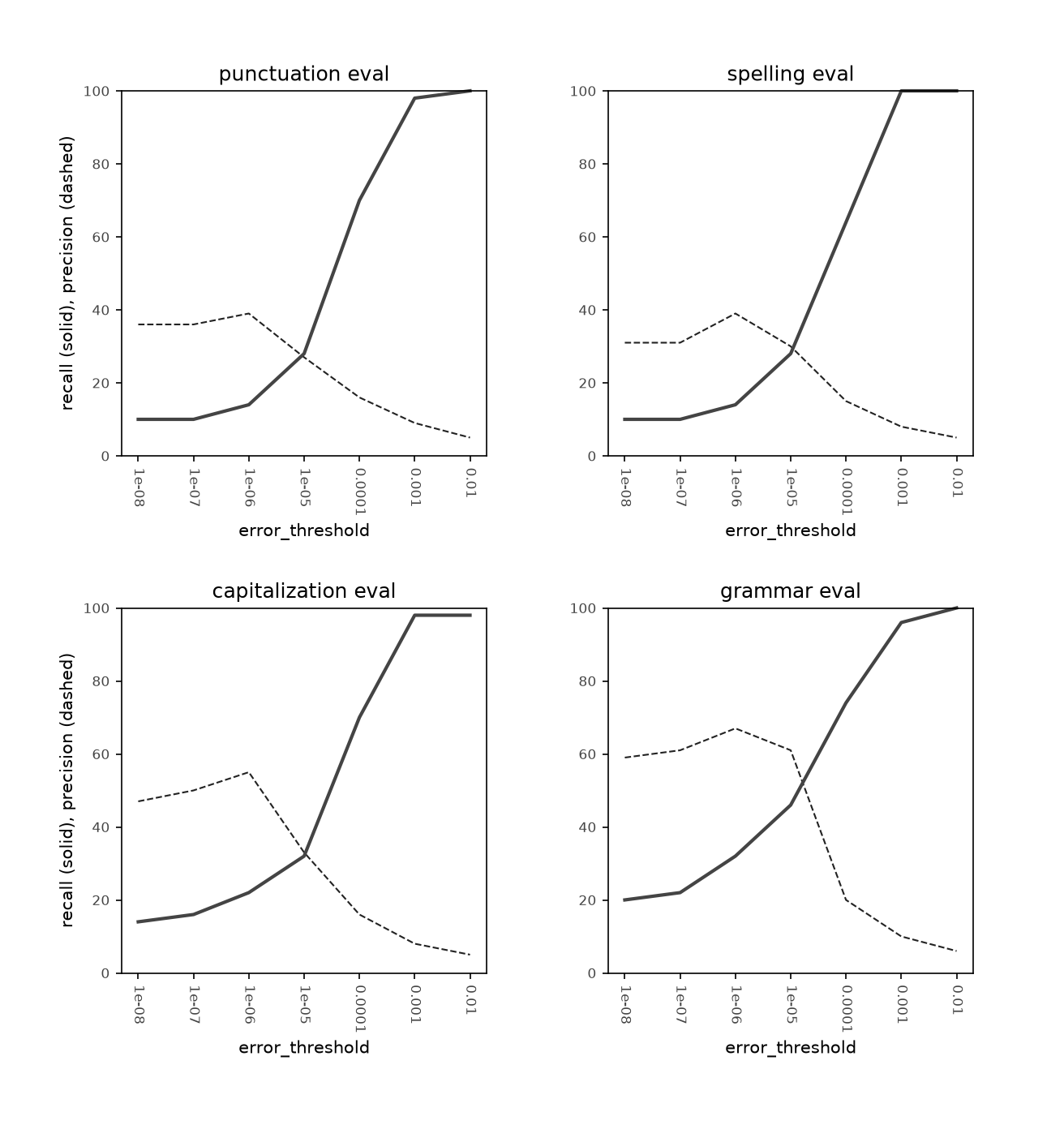
I added plotting code to the reporting function. The patterns that may have been apparent in the tables really pop out in the plots (at least to my brain). More than four rows in a table quickly turns into a wall of numbers. Especially as we start systematically varying aspects of the models, plots will help those patterns emerge.
The plots show how recall starts in the single digits on the left and climbs to 100% on the right. Precision starts middle-to-low and climbs slightly before it starts descending to settle in at the single digits on the right.
There is a nice crossover point at around 1e-5 for each of the evals, where recall and precision are roughly balanced. It can be shifted either direction to favor one over the other.
Scaling up bookkeeping
As is evident from the escalating version numbers, there is a rapidly-multiplying set of permutations of corpus/tokenizer/model/error threshold. The registry system I started using during the previous post required entering the version numbers of proofreader components in several different locations, which already resulted in a couple of errors.
To get around this, I upgraded all the registries so that instead of just cataloguing the characteristics of a model, they actually linked to the model itself. That way the characteristcs, such as tokenizer version in use by a given Markov model, could be read from the model itself, rather than manually entered into an informational dictionary. This saved a lot of potential errors. As a bonus, it eliminates several of the steps necessary for specifying and testing a new model, which streamling I'm really appreciating right now.
Shrinking the code by refactoring
Another scaling consideration is that I had started out using a lot of individual scripts to create and train each individual model version. I had also been largely copy/pasting 99% of the code for each new proofreader. It was time to clear this up.
Object-oriented programming made this possible. I made sure everything was a class, including the random baseline model which was trivial and didn't need to be one. Then I collapsed all of the parameters necessary to create each new element into the class' initialization arguments. At that point, it was possible to define and create the model object in a single call to the class. These model creation calls became the new registry, for example
registry = {
    "00": SecondOrderMarkovModel(
        version="00",
        tokenizer_version="04",
        corpus_versions=["00"],
        description="2nd-order Markov",
    ),
    "01": SecondOrderMarkovModel(
        version="01",
        tokenizer_version="04",
        corpus_versions=["00", "01"],
        description="2nd-order Markov",
    ),
    "02": SparseSecondOrderMarkovModel(
        version="02",
        tokenizer_version="00",
        corpus_versions=["00", "01"],
        description="Sparse 2nd-order Markov",
    ),
...
Registries are still Python dictionaries. This change also required some careful thinking about when models would actually be loaded into memory and when training would kick off for untrained models. Collectively the models are too big to all reside in memory at once. (The largest are 12GB on disk, and I only have 16 GB of RAM.) If they were to all load when the registry gets loaded that would overload things. Also, training times for some models are many hours long. Kicking these off unintentionally would be undesirable. I made sure that loading and training were lazy, that is, that they don't train or load until they absolutely have to in order to calculate probabilities.
Extending to second-order models
The contraints of memory and training time become more intense when working with second-order models. Back when these were dense arrays, we saw how memory demands jumped from the square to the cube of alphabet size. Infeasibly large for most of the alphabets the tokenizers are working with. There is a similar dynamic with dictionaries. The number of unique token triples outnumbers the number of unique token pairs by many times. Not quite by a factor of the alphabet size, since not all possible triples occur, but by some significant fraction of it. We can no longer ignore the constraints of memory.
Memory constraints exacerbate another problem, training time. Once physical memory is overextended, the system starts swapping in disk space to cover the difference, which is desperately, painfully slow in comparison. There are other drags on training time that bear investigation later, but this is the one that hurts the most.
OK-but-not-great: Moving to SQLite databases
The first thing I tried was tracking the bigram and trigram counts in a SQLite database, rather than a Python dictionary. I created a new variant of the second-order Markov model that was still sparse, but added or incremented the count of each tuple in a database row. This file shows how I implemented it.
Using a database has the advantage that it can grow much larger than my RAM, as big as my whole hard drive if necessary. Sadly it comes with the disadvantage that it is reading to and writing from disk. It makes training very slow, even after I attempted to do some optimizations for speed. Database optimization is a dark art, and it's possible that there are some configurations that would make it snappy, but I couldn't figure them out. Even more problematic for the proofreading application, it looked like the reading would be sluggish too. That means even if I were patient enough for the training, the user experience of the final tool would be clunky and slow. I put a pin in this option. The lesson I (re)learned from this is that if you want something to be very fast, keep it all in RAM. It's worth noting that the speedy key-value stores backing serious architectures (e.g. DynamoDB) are all made to read from RAM.
Better: Size-limiting the tuple dictionaries
I went back to dictionaries with the goal of keeping them just small
enough to fit in RAM. The new constrained second-order model
has an upper limit on the number of trigrams it can track (these far
outnumber the number of bigrams). Once it hits that limit it has to thin
them out, and reduce them back down to a more manageable size.
These two parameters, max_dict_size and max_dict_size_after_shrink,
help determine exactly how the model behaves, and become part of
its short list of specification, also known as hyperparameters.
The way the memory-constrained model stays trim is to drop triples that are only rarely observed. If a token triple has been seen a thousand times, it is clearly a common occurrence in the world. But if it has only been seen once, there is a good chance that it is a fluke. So if we have to drop something, it makes sense to let it be the least-observed items. This amounts to a lossy compression of the model, chopping off some of the less critical information while preserving the most important bits.
The model goes about this systematically by first dropping all the
triples that have been seen once. Then it checks whether it has fallen
below max_dict_size_after_shrink. If not, it drops everything it has
only observed twice. This process repeats until the model gets small
enough to pass the reduced size threshold. Then it resumes training.
After some exploration, trial, and error showed that for my computer
(16GB, Apple M2 Pro) max_dict_size = 5e7 and
max_dict_size_after_shrink = 4e7 gave maximum model size without
bogging down training. That works out to roughly 1 GB per 10 million
tuples, or 100 bytes per tuple. That still feels pretty inefficient to
me, since the count value will be at most an 8-byte integer. It looks
like most of the space goes to the key (a tuple of integers) and any
overhead the python dictionary object occupies. I'm noting that
space efficiency is an area to explore for future improvements.
Performance of second order models
But the good news is that I can now train second-order Markov models on arbitrarily large data sets! And the bad news is that it doesn't seem to help much, at least not at first. A second-order model with an alphabet size of 20k, trained on a library of 14.4 thousand books never gets precision into the double digits.
| version | description | model | tokenizer | alphabet | books | error cutoff |
|---|---|---|---|---|---|---|
| 47 | Constrained 2nd-order Markov | 21 | 05 | 20k | 14382 | 1e-08 |
| 48 | Constrained 2nd-order Markov | 21 | 05 | 20k | 14382 | 1e-07 |
| 49 | Constrained 2nd-order Markov | 21 | 05 | 20k | 14382 | 1e-06 |
| 50 | Constrained 2nd-order Markov | 21 | 05 | 20k | 14382 | 1e-05 |
| 42 | Constrained 2nd-order Markov | 21 | 05 | 20k | 14382 | 0.0001 |
| 51 | Constrained 2nd-order Markov | 21 | 05 | 20k | 14382 | 0.001 |
| 52 | Constrained 2nd-order Markov | 21 | 05 | 20k | 14382 | 0.01 |
| version | capitalization | grammar | punctuation | spelling |
|---|---|---|---|---|
| 47 | (8) 94 | (10) 92 | (8) 94 | (8) 98 |
| 48 | (8) 94 | (10) 92 | (8) 94 | (8) 98 |
| 49 | (8) 94 | (10) 92 | (8) 94 | (8) 98 |
| 50 | (8) 94 | (10) 96 | (8) 94 | (8) 98 |
| 42 | (8) 96 | (10) 96 | (8) 96 | (8) 98 |
| 51 | (7) 100 | (8) 98 | (7) 96 | (7) 100 |
| 52 | (6) 100 | (7) 100 | (5) 100 | (5) 100 |
Performance values are shown as: (precision %) recall %
This means that too many things are new to it. It gets shocked every time it turns a corner because it has never seen that exact combination of tokens before.
Experimenting with smaller dictionaries in second-order models
One way to help the model get surprised less easily is to reduce its world to a more manageable size. With a tokenizer vocabulary of 20,000, there are 8 trillion possible triples. But at a vocab size of 1,000 that comes down to 1 billion possibilities. And at a vocab size of 200, that becomes a measly 8 million possible triples.
This is reflected in the second-order model's performance as vocabulary shrinks. Recall falls, meaning that it misses more and more of the actual errors. But precision climbs, meaning that when it does declare something an error its more likely to be right.
| version | description | model | tokenizer | alphabet | books | error cutoff |
|---|---|---|---|---|---|---|
| 42 | Constrained 2nd-order Markov | 21 | 05 | 20k | 14382 | 0.0001 |
| 53 | Constrained 2nd-order Markov | 26 | 06 | 10k | 14382 | 0.0001 |
| 54 | Constrained 2nd-order Markov | 27 | 07 | 5k | 14382 | 0.0001 |
| 55 | Constrained 2nd-order Markov | 28 | 08 | 2k | 14382 | 0.0001 |
| 56 | Constrained 2nd-order Markov | 29 | 09 | 1k | 14382 | 0.0001 |
| 57 | Constrained 2nd-order Markov | 30 | 11 | 500 | 14382 | 0.0001 |
| 58 | Constrained 2nd-order Markov | 31 | 12 | 200 | 14382 | 0.0001 |
| 59 | Constrained 2nd-order Markov | 32 | 13 | 100 | 14382 | 0.0001 |
| version | capitalization | grammar | punctuation | spelling |
|---|---|---|---|---|
| 42 | (8) 96 | (10) 96 | (8) 96 | (8) 98 |
| 53 | (10) 92 | (12) 90 | (9) 88 | (9) 92 |
| 54 | (14) 88 | (13) 68 | (11) 76 | (12) 82 |
| 55 | (25) 72 | (26) 56 | (19) 60 | (21) 68 |
| 56 | (51) 56 | (27) 24 | (40) 46 | (36) 62 |
| 57 | (66) 46 | (50) 14 | (58) 44 | (49) 58 |
| 58 | (62) 26 | (50) 6 | (76) 32 | (69) 48 |
| 59 | (75) 18 | (100) 4 | (78) 14 | (62) 32 |
Performance values are shown as: (precision %) recall %
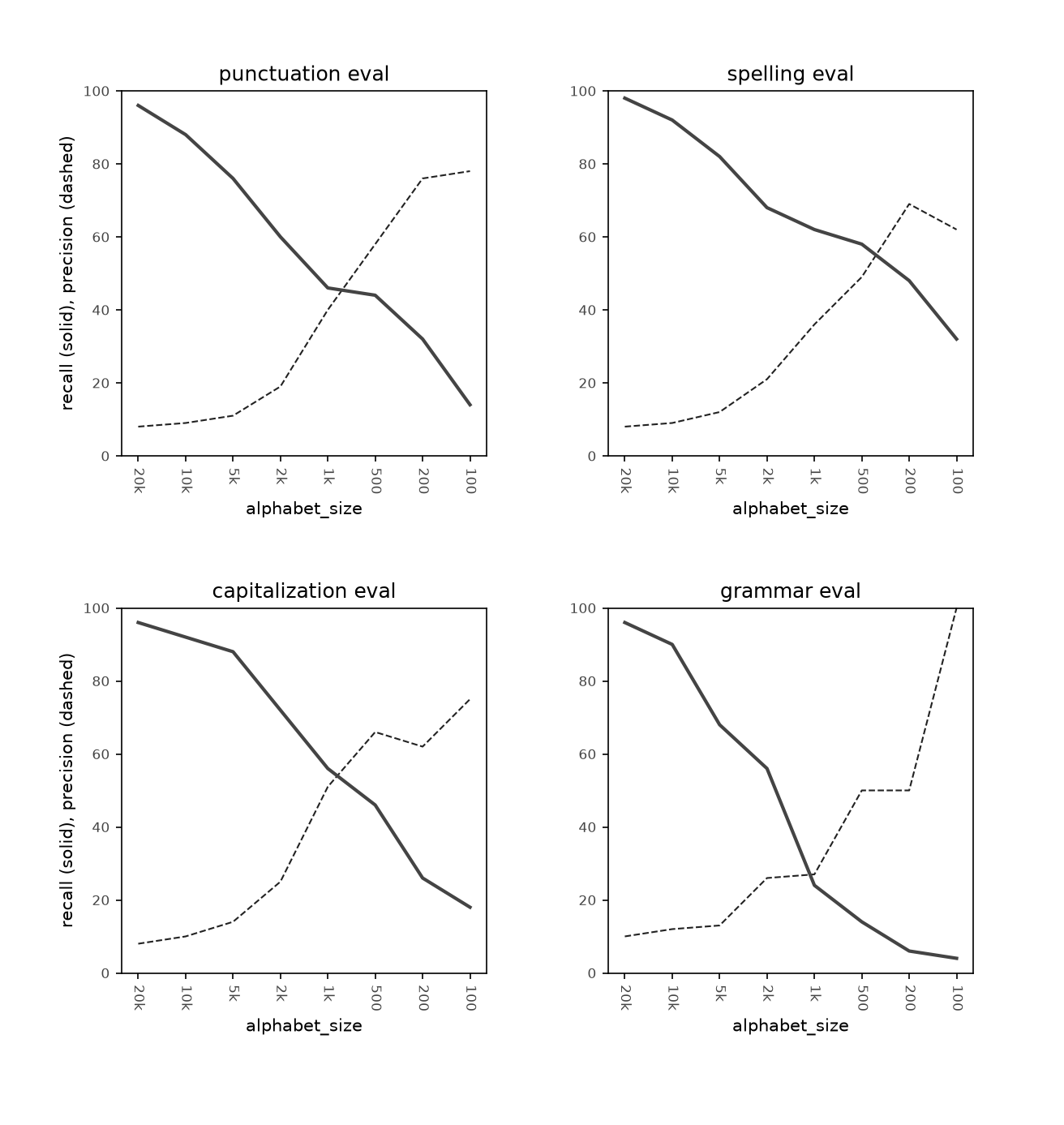
This is huge progress! Having a model at roughly the 50/50 precision/recall mark as this one is means that it catches half of the errors and that of the errors it reports, half are legitimate. It's still not good enough for prime time, but this is a very solid step forward.
Experimenting with smaller dictionaries in first-order models
In the prior post, we saw this same pattern in performance with changes in dictionary size in first-order models, but now we are in a better position to revisit it. There are a broader set of dictionaries to work with, larger training data sets, a better guess at a good error threshold, visual reporting, and a way to handle inconveniently large models.
Matching the second-order model set above, this gets a similar pattern.
| version | description | model | tokenizer | alphabet | books | error cutoff |
|---|---|---|---|---|---|---|
| 60 | Sparse 1st-order Markov | 05 | 05 | 20k | 14382 | 0.0001 |
| 61 | Sparse 1st-order Markov | 08 | 06 | 10k | 14382 | 0.0001 |
| 62 | Sparse 1st-order Markov | 09 | 07 | 5k | 14382 | 0.0001 |
| 63 | Sparse 1st-order Markov | 10 | 08 | 2k | 14382 | 0.0001 |
| 64 | Sparse 1st-order Markov | 11 | 09 | 1k | 14382 | 0.0001 |
| 65 | Sparse 1st-order Markov | 12 | 11 | 500 | 14382 | 0.0001 |
| 66 | Sparse 1st-order Markov | 13 | 12 | 200 | 14382 | 0.0001 |
| version | capitalization | grammar | punctuation | spelling |
|---|---|---|---|---|
| 60 | (17) 76 | (21) 78 | (16) 72 | (17) 70 |
| 61 | (21) 68 | (23) 70 | (19) 66 | (19) 62 |
| 62 | (23) 54 | (22) 52 | (22) 54 | (23) 52 |
| 63 | (31) 50 | (24) 30 | (28) 46 | (28) 44 |
| 64 | (47) 42 | (30) 16 | (46) 42 | (37) 36 |
| 65 | (68) 34 | (73) 16 | (68) 38 | (46) 24 |
| 66 | (75) 18 | (100) 6 | (87) 26 | (69) 18 |
Performance values are shown as: (precision %) recall %
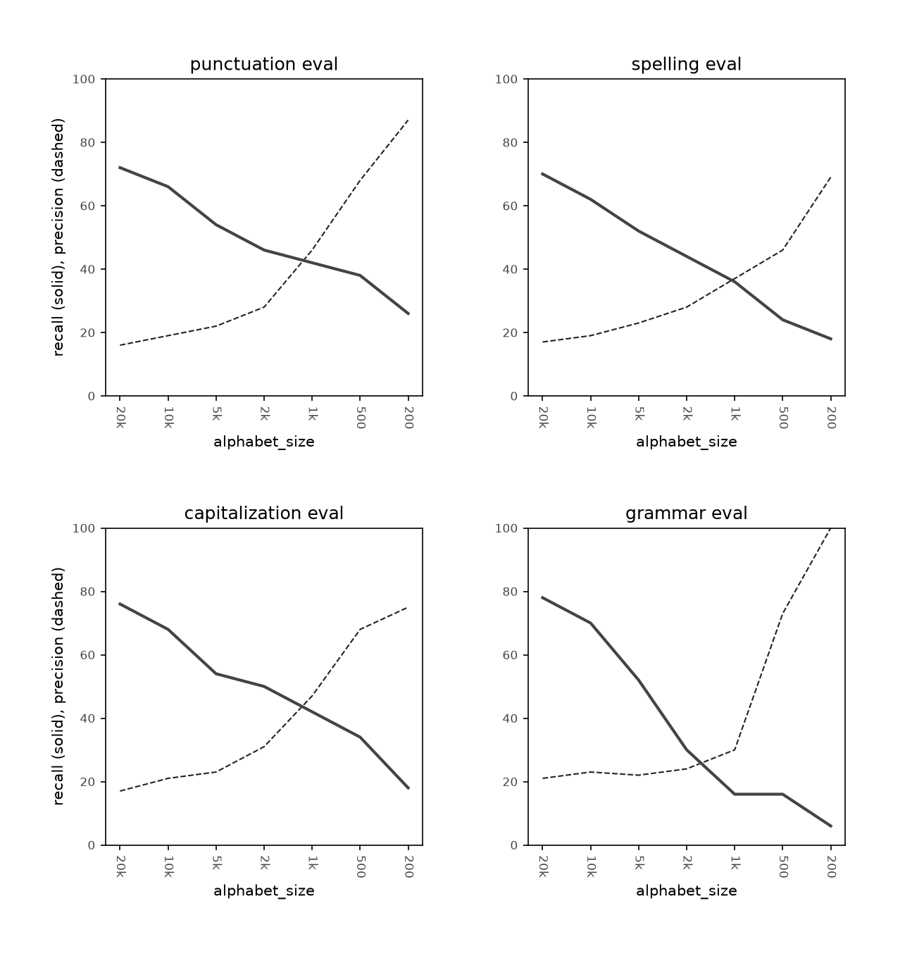
Again, the crossover point where precision equals recall tended to be in the neighborhood of a dictionary size of 1000. This is very promising. It suggests that we have a lot of freedom to adjust models' behavior and sensitivity by tweaking hyperparameters like alphabet size.
It's also convenient, because it appears that, rather than using tokenizers with very large vocabularies, smaller ones are proving more effective with Markov models. This will save a mountain of memory space.
Eval expansion: Adding to grammar/word choice
It's time again to invest the tedious work to expand the eval set. Rather than kick off a new eval type, I chose to expand an existing eval with an additional 50 examples. This time I used a different text; instead of continuing with Frankenstein, I pulled snippets from Call of the Cthulhu. It's prose is a little more modern and less stilted, so it will help make the evals more representative.
Next steps
This last round of improvements have been especially gratifying. We're no long just laying foundations. The beginnings of the proofreader itself are starting to become visible. Performance is not great but is good enough to be interesting.
The next round will focus on model enhancements. Of course there will be continued work on enriching the training data, refactoring to make the code as clear and usable as possible, adapting to the hardware limitations of artisanal development, building out the evals, and systematic exploration of varying hyperparameters. But these fundamentals are now strong enough to support exploring novel models.
See you next time.